Numerical Methods

for Calculus & DE

	MA3457/CS4033 Homework: Additional Problems

B'14 Term 2014-2015 Sections B01/B01 Mon, Tue, Thu, Fri - 2:00 pm

[1]. Verify that the polynomials

p(x) = 5x^3 - 27x^2 + 45x - 21 & q(x) = x^4 - 5x^3 + 8x^2 - 5x + 3

interpolate the data

x | 1 2 3 4
------------
y | 2 1 6 47

and explain why this does not violate the uniqueness part of the Theorem on existence of polynomial interpolation.

[2]. Given the data

(x1, y1) = (0, 1); (x2, y2) = (1, 9); (x3, y3) = (2, 23); (x4, y4) = (4, 93); (x5, y5) = (6, 259)

construct the divided-difference table. Using Newton's interpolation polynomial, find an approximation to x = 4.2.

[3]. Using the class 5- and 9-point data for the Runge's function with a = 25 on the interval [-1, 1], find corresponding divided-difference tables.

[4]. Given the data

x = 0.70 => sinx = 0.6442176872; cosx = 0.7648421872
x = 0.71 => sinx = 0.6518337710; cosx = 0.7583618759

find approximate values of sin0.705 and cos0.702 by linear interpolation. What is the error?

[5]. An interpolating polynomial of degree 20 is to be used to approximate exp(-x) on the interval [0,2]. How accurate will it be?

[6]. Consider the data points from the lecture (Class 3)

(x1, y1) = (-2, 4); (x2, y2) = (-1, -1); (x3, y3) = (0, 2); (x4, y4) = (1, 1); (x5, y5) = (2, 8)

and construct for them a natural cubic spline (i.e., take a0 = a4 = 0).

Guidelines: Three equations for a1, a2, a3 could be produced from the class formula (CS2). Substitution of the values of a1, a4, and yi (i = 1, ..., 5) yields the linear system of three equations for a1, a2, a3 - this system could be solved with a suitable MATLAB function (e.g., for Gauss elimination). All the resulting values of ai are then substituted into the class formula (CS3). This leads to the cubic spline S(x) in the form of the class formula (CS1) - four cubic polynomials for each sub-interval.

[7]. Using the Forward Difference Formula (FDF), the Backward Difference Formula (BDF), and the Central Difference Formula (CDF), approximate y' (1) if x = [0 1 2] and y = [1 3 9].

[8]. Derive the approximation formula

f'(x) ~ (1/2h)[4f(x + h) - 3f(x) - f(x + 2h)]

and show that its error term is of the form (1/3)h^2f '''().

[9]. Solve problem [7] using Richardson extrapolation (RE) and considering the expanded vectors x = [-1 0 1 2 3], y = [1/3 1 3 9 27].

[10]. Use RE to estimate the first derivative of

at x = 0.5. Compare the result with y '(0.5).

[11]. Derive the normal equations of the Quadratic Least Squares Approximations.

[12]. Consider an approximation of a given function s(x) with a quadratic function p(x) = ax^2 + bx + c on the interval [-1, 1] and derive the normal equations for a, b, and c - calculate the coefficients in matrix P and the components of vector q.

[13]. Find the Quadratic Least Squares Approximation to f(x) = exp(x) on the interval [-1, 1] in terms of the Legendre polynomials.

[14] (Optional). Find the Quadratic Least Squares Approximation to f(x) = exp(x) on the interval [-1, 1] in terms of the Chebyshev polynomials.

[15]. Compute an approximate value of

by using the Composite Trapezoid Rule with three points and compare with the actual value of the integral.

[16]. Obtain an upper bound on the absolute error when computing

by means of the Composite Trapezoid Rule using 101 equally spaced points.

[17]. Answer the question in problem [C21] applying an analytical solution rather than a computational experiment.

[18]. Find a bound on the error in the approximation value of

obtained using Composite Simpson's Rule with h = 0.25.

[19]. Approximate the integral

using Gaussian quadrature with n = 3 and compare the result to the exact value of the integral.

[20] (Optional). Derive the Gaussian Quadrature rule for n = 2 by ensuring the rule is exact for the Legendre polynomials on the interval [-1, 1].

[21]. Solve the following IVP:

y' = yx^2 - 1.2y, where y(0) = 1

over the interval from x = 0 to x = 2 analytically and using Euler's method with h = 0.5 and 0.25. Calculate average errors of the approximations obtain numerically.

[22]. Use the fourth-order Runge-Kutta method with h = 0.5 to solve the IVP in [21].

[23]. Use the fourth-order Runge-Kutta method with h = 1.0 and 0.5 to solve the IVP:

y' = (t - y)/2,

where 0 < t < 3 and y(0) = 1

[24]. The first-order ODE governing unsteady heat transfer from a lumped mass gives the temperature T as:

T' = f(t, T) = -(T^4 - T^4)

With the initial temperature T(0) = 2500 C, T = 250 C, and = 2.0 x 10^-12, and assuming that the derivative function does not depend explicitly on t, find, using the fourth-order Runge-Kutta method, the temperature in 3 s. Use the time step of 1 s.

[25]. The electrostatic potential between two concentric spheres is given by

The potentials of the inner sphere of radius 1 and of the outer sphere of radius 2 are 10 and 0 respectively; this gives the boundary conditions y(1) = 10, y(2) = 0. Derive the equivalent system of four 1st order ODE's. Then go to problem [C40].

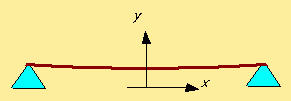
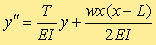
[26]. Consider a bean that is freely hinged at its ends (e.g., at x = 0 and x = L) with a uniform transverse load w and tension T:

In this case, the deflection y(x) of the beam is described by the BVP

0 < x < L, y(0) = y(L) = 0. (The physical parameters of the beam are the modulus of elasticity E and the central moment of inertia I.)

Derive the equivalent system of four 1st order ODE's for the following parameters: L = 100, w = 100, E = 10^7, T = 500, I = 500. Then go to problem [C41].

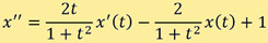
[27]. Derive the equivalent system of four 1st order ODE's for the boundary value problem

with x(0) = 1.25 and x(4) = -0.95 over the interval [0, 4]. Then go to problem [C42].

[28]. Consider the BVP

y" = - y,

where y(0) = 0, y(1) = 1.

Set up and solve the tridiagonal system that arises from the finite-difference method when h = 1/4.

[29]. Solve the BVP

y" = 1 - y,

where y(0) = -1, y(2) = 1

using the finite-difference method and applying n = 4.

[C1]. Test Lagrange_coef on Example 2a (Section 3.1) and Problems 3.1.5a and 3.1.5b: show that the procedure generates the coefficients obtained in these problems analytically.

[C2]. Test Lagrange_Eval on Example 2b (Section 3.1) and Problems 3.1.5a and 3.1.5b: show that the obtained values are identical to the ones derived from the final polynomials analytically.

[C3]. Test Newton_coef on Example 1 (Section 3.3) and Problems 3.3.1a and 3.3.1b: show that the procedure generates the coefficients obtained in these problems analytically.

[C4]. Test Newton_Eval on Example 1 (Section 3.3) and Problem 3.3.1a and 3.3.1b: show that the obtained values are identical to the one derived from the corresponding polynomial analytically.

[C5]. Add graphical visualization of the obtained interpolation polynomials to your MATLAB scripts employing both the Lagrange and Newton forms. Test the graphical output on the examples considered in class.

[C6]. Compose a MATLAB procedure computing and plotting Chebyshev points. Test the procedure on the Runge's function with a = 25 on the interval [-1, 1] and make sure that the x-coordinates generated by the numerical values quoted in the lecture (Class 4).

[C7]. Demonstrate (graphically) the performance of the course Lagrange and Newton interpolation functions in comparison with the built-in MATLAB procedure interp1 for the Runge's function with a = 5, 25, and 100 on the interval [-5, 5] with equally spaced and Chebyshev points.

[C8]. Apply Spline_test to get a cubic spline interpolation for the "bulge-flat" data considered in class:

x = [ -2 -1.5 -1 -0.5 0 0.5 1 1.5 2 ]
y = [ 0 0 0 0.87 1 0.87 0 0 0 ]

Plot the resulting spline interpolation on the same graph with the curve generated by Newton interpolation.

[C9]. Apply Spline_test to get a cubic spline interpolation for the "noisy straight line" data considered in class:

x = [ 0 0.2 0.8 1 1.2 1.9 2.0 2.1 2.95 3 ]
y = [ 0.01 0.22 0.76 1.03 1.18 1.94 2.01 2.08 2.90 2.95 ]

Plot the resulting spline interpolation on the same graph with the curve generated by Newton interpolation.

[C10]. For x = [x(1) x(2) ... x(n)], MATLAB's built-in function diff(x) gives a vector (of length n-1) consisting of the differences between successive elements of x, i.e., [x(2)-x(1) x(3)-x(2) ... x(n)-x(n-1)]. Thus, the ith element of diff(y)./diff(x) is the forward difference approximation to dy/dx at x(i).

• Write a MATLAB procedure FBC_Diff based on the diff(x) function and performing numerical differentiation using the FDF, BDF, and CDF.
• Test FBC_Diff on the example considered in class [i.e., given (x1, y1) = (2, 4), (x2, y2) = (3, 8), (x3, y3) = (4, 16), approximate f'(x2)] and make sure that the MATLAB procedure produces the same results as obtained manually.
• Use FBC_Diff to estimate the derivative of y = lnx at x = 2 if x(1) = 1.0, x(2) = 1.5, x(3) = 2.0, x(4) = 2.5, and x(5)=3.0.

[C11]. Compose a script calling Lin_LS, computing the total squared error, and plotting the data points along with the generated approximating line. Test Lin_LS on the class examples with four data points.

[C12]. Use Lin_LS to find the Linear Least Squares Approximation (equation of the line, its graph, total square error) for the points x = [4 9 16], y = [2 3 4].

[C13]. Compose a script calling Quad_LS, computing the total squared error, and plotting the data points along with the generated approximating curve. Test Lin_LS on the class example (5 data points on a chemical reaction).

[C14]. Use Quad_LS to find the Quadratic Least Squares Approximation (equation of the curve, its graph, total square error) for the points x = [-1 0 1 2], y = [1/3 1 3 9].

[C15]. Compose the MATLAB function Cubic_LS giving the Cubic Least Squares Approximation. Supplement it with a script calling this function, computing the total squared error, and plotting the data points along with the generated approximating curve. Test Cubic_LS on the on the class example (11 data points on a population logistic model) and on other examples you find suitable.

[C16]. Use Cubic_LS to find the Cubic Least Squares Approximation (equation of the curve, its graph, total square error) for the data points of the logistic model (problem [C15]) with only 6 points on the interval [0,1].

[C17]. The MATLAB built-in function polyfit finds the coefficients of the polynomial of specified degree that best fits a set of data, in a least squares sense. The output of polyfit can be used with the function polyval to obtain error bound on the predictions. Compose a script calling these functions and find the degree n (4 <= n <= 8) of the polynomial which appears to be the best approximation for the logistic model (see problem [C15]) on the interval [-1, 1].

[C18]. Compose a MATLAB script visualizing the first six (P to P) Legendre polynomials on the interval [0, 1].

[C19]. Compose a MATLAB script visualizing the first six (T to T) Chebyshev polynomials on the interval [0, 1].

[C20]. Compose a script calling Trap and computing approximations to the definite integrals of given functions on the given intervals and with the specified number of subintervals.

[C21]. Test Trap for function f(x) = 1/x and make sure that you get the numerical results presented in class. Provided that the exact value of the integral is ln(2) ~ 0.6931..., perform computational experiment to find out with what n this function can generate 4 decimal digits of accuracy.

[C22]. Compose the MATLAB function Simp performing numerical integration of function f(x) on the interval [a, b] using the Composite Simpson Rule for any even n. Then write another script plotting f(x) on [a, b] and calling Simp. Test the procedure and make sure it works properly.

[C23]. Use the script developed in [C22] to integrate function f(x) = sin(x^2) on the interval [0, ]. Provided that the accurate numerical value of this integral is ~ 0.77265..., perform computational experiment to find out with what n your MATLAB procedure generates these 5 decimal digits of accuracy. Give a qualitative explanation of why n is large.

[C24]. Compose a script calling Romb and computing approximations to the definite integral of a given function on the given interval and with the specified number of stages of Romberg Integration. Test the procedure with any suitable examples. Apply Romb, Simp, and Trap to the example considered in class (integration of y = 1/(1 + x^2) on the interval [-1, 1]) and find with what n all three techniques provide approximation accurate to four decimal places.

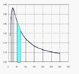
[C25]. Apply Romb to the function y = 1/(x^p), where p = 1, 3, and 5, integrating it on the interval [1, 100]. At which step d of Romberg Integration this MATLAB function gives the accuracy of 4 correct decimal digits for each of the values of p?

[C26]. Apply Romb to the function y = x^0.1 in the range 0 to 1. Keeping in mind that the exact solution to four decimal places is 0.9090, experiment with the procedure to get three different combinations of d (i.e., steps in Romberg Integration) and n (i.e., the intervals in Simpson's Rule) required to get 0.9090.

[C27]. Compose a script calling Gauss_quad and computing approximations to the definite integral of a given function on the given interval with the specified number of Gaussian points. Test Gauss_quad on the example considered in class (integration of y = 1/x on the interval [1, 2] and y = exp(-x^2) on the interval [0, 2]).

[C28]. Apply Gauss_quad and Romb to the function y = sqrt(x^2 - 4) integrating it on the interval [2, 3] and to the function y = (x^3 + 1)^(1/3) integrating it on the interval [0, 3]. Give a qualitative comparative characterization of performances of both functions with y and y.

[C29]. Reproduce all computational experiments with Trap, Simp, Romb, and Gauss_quad shown in class for

y = sin(x^2),
y = x^2(x - 1)^2(x - 2)^2(x - 3)^2(x - 4)^2,
y = x^0.01,
and y = 1/[1 + (230x - 30)^2]

and identify the procedure using the least n and the least CPU time to get the accuracy up to four decimal places.

[C30]. Apply Gauss_quad, Romb, Simp, and Trap to evaluate the Fresnel integrals:

The exact values, to 7 decimal places, are C(1) = 0.7798934 and S(1) = 0.4382591. Try to get these values by each of the above MATLAB functions: how many intervals are required for Simp and Trap? how many points for Gauss_quad? how many stages for Romb?

[C31]. Compose a script calling Euler to solve a given initial value problem. The script should visualize the obtained points of numerical solution and the curve representing the analytical solution (if the latter is available). Test Euler on the example considered in class (y' = x + y, y(0) = 2 on [0, 2]) for n = 5, 10, and 20.

[C32]. Apply Euler to the initial value problem y' = yx^(-2), y(1) = 2 on [1, 2] for n = 20, 50, and 100 and compare the numerical results with the analytical solution.

[C33]. Compose the MATLAB function Taylor_2 solving a given initial value problem using the 2nd order Taylor method. Then write another script calling Taylor_2 and plotting the obtained points of numerical solution and the curve representing the analytical solution (if the latter is available). Test Taylor_2 on the example considered in class (y' = -2xy, y(0) = 2 on [0, 1]) for n = 5, 10, and 20.

[C34]. Apply Taylor_2 to the initial value problem y' = 3yx^2, y(0) = 1 on [0, 1] for n = 20, 50, and 100 and compare the numerical results with the analytical solution.

[C35]. Compose a script calling RK2 to solve a given initial value problem. The script should visualize the obtained points of numerical solution and the curve representing the analytical solution (if the latter is available). Test RK2 on the example considered in class (y' = 1 - 2xy, y(0) = 0 on [0, 1]) for n = 10.

[C36]. Compose a script calling RK4 to solve a given initial value problem. The script should visualize the obtained points of numerical solution and the curve representing the analytical solution (if the latter is available). Test RK4 on the examples considered in class: y' = x + y, y(0) = 2 on [0, 1] for n = 5; and (1 + x^2)y' + 2 xy = cosx, y(0) = 0 on [0, 2] for n = 8.

[C37]. Apply RK2 to the initial value problem y' =3y/x, y(1) = 1 on [1, 2]. Find an analytical solution for x = 2 and determine n with which RK2 provides for this point a numerical solution with 2 correct decimal digits.

[C38]. Apply RK4 to the initial value problem y' =3 + 5sinx + 0.2y, y(0) = 0 on [0, 10] and find the minimal number of intervals n providing 3 correct decimal digits for the solution at x = 10, i.e., y = 135.917.

[C39]. Analyze and adapt to your MATLAB environment the functions BVP_shooting and RK4_sys. Run computation for the example considered in class:

y(0) = 2, y(1) = 5/3 using the fivp_sys function defining the right-hand sides of the equivalent ODE-IVP system of order 1. Make sure that you get the right numerical results for n = 10.

[C40]. Use BVP_shooting and RK4_sys to get a numerical solution for problem [25]. Hint: Function fivp_sys should be used and reformulated accordingly.

[C41]. Use BVP_shooting and RK4_sys to get a numerical solution for problem [26]. Hint: Function fivp_sys should be used and reformulated accordingly.

[C42]. Use BVP_shooting and RK4_sys to get a numerical solution for problem [27]. Hint: Function fivp_sys should be used and reformulated accordingly. Visualize the numerical solution on one graph with the analytical solution:

[C43]. Revise the function BVP_shooting to compose the function BVP_shooting_b which handles the general boundary condition y'(b) + cy(b) = yb. Then solve the BVP in [C39] with y(0) = 1, y'(1) + y(1) = 0. Show graphically that the obtained numerical solution is indistinguishable from the exact solution y = (x^4 - 3x^2 - x + 6)/6.

[C44]. Analyze and adapt to your MATLAB environment the functions BVP_FD and Trid_Thomas. Run computation for the example considered in class (y" = 2y' - 2y, y(0) = 0.1, y(3) = 0.1exp(3)(cos3). Comparing with the data in the handout, make sure that you get the right numerical results for n = 300. Determine (by a computational experiment) the smallest n which gives two correct decimal digits of the numerical solution.

[C45]. Adapt the pair of the MATLAB functions, BVP_FD and Trid_Thomas, to solve Problem 11.3.3b.

[C46]. Adapt the pair of the MATLAB functions, BVP_FD and Trid_Thomas, to solve Problems 11.3.3c.

Course Information | Homework Assignments | Mini Projects | Test Preview | Announcements & Hints

vadim@wpi.edu

Last modified: Fri, Dec 12, 2014