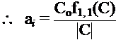
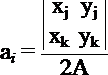
2-D Linear Elements: Linear Triangles
![]()
Complete linear polonomial. That is, a constant term and linear terms in x and y
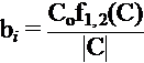
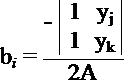
2-D Linear Elements: Linear Triangles
![]()
Complete linear polonomial. That is, a constant term and linear terms in x and y
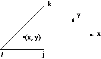
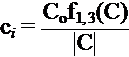
Trianglar elements can take any orientation and satisfy continuity requirements involving adjacent elements
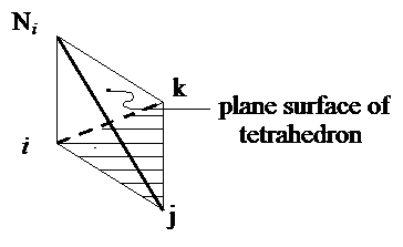
Use CCW convection (Node "i" to "j" to "k" form right-hand rule for outward normal).
![]()
![]()
for local node numbering
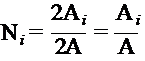
Solve for coefficients ![]()
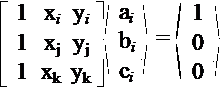
or
Then soln of coefficients
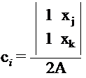
 only significant entries are
in
only significant entries are
in ![]() column 1
column 1
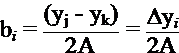
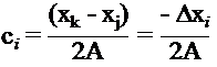
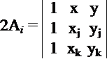
Recall : Area of triangle is ![]()
 ;
;  ;
; 
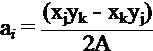
![]()
![]()
Where the 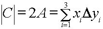
CCW ordering gives a positive (+) area
note: 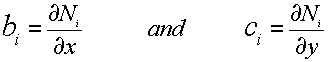
Pictorially, Ni
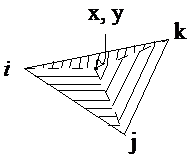
Look at a point (x, y) in ![]()
![]()
 the
the ![]() are the
"area" coordinates
are the
"area" coordinates
There are multiple ways to calculate the area of a triangle. The following description gives a general 3D solution to the situation. (Triangle Area)
The following link provides a table for integration formulaes for linear triangles (Integration Formulae)
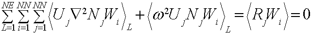
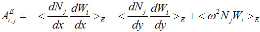
Examine a 2-D Helmholz Eqn
![]()
![]()
Use same procedure as in 1-D case.
1.) Substitute for U a trial fxn

![]() constant coeff.
constant coeff.
![]()
![]()
![]()
2.) Force ![]() to zero in "weak
form"
to zero in "weak
form"
a.)
multiply by weight fxn ![]()
![]()
b.) integrate over entire domain and force to zero
![]()
3.) Discretize domain into subregions (elements)
4.) Select Basis function: here we use Linear triangles with Ni just calculated.
5.) Integrate by parts which is the vehicle or mechanism for applying B.C.
(Use implied summation)

Remember that the
Uj term is also part of the integrated by parts term.
6.) Select Weighting functions and
functional coefficients (if used) i.e.
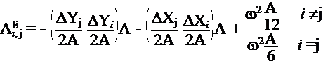
7.) Assemble Matrices
for L = 1 : NE Rhs(iGlobal)
= Rhs(iGlobal) + 0 End
% (I loop)
End % (L
loop) 
![]()
c
c calculate Dx, D y,
and area
c
area = 0;
for i = 1 : 3
j = in( mod(i,3) +1, L);
k = in( mod(i+1,3)+1, L);
dx(i) = x(j) - x(k);
dy(i) = y(j) - y(k);
area = area + x(in(i,L))*dy(i);
end
area = area / 2.;
for i = 1 : 3
iGlobal = in(I,L);
for
J = 1 : 3
jGlobal = in(J,L);
Bcol = diag + (jGlobal - iGlobal);
AIJ = -(dy(j)*dy(i) + dx(j)*dx(i))/(4*area);
if i == j
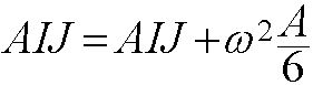 ;
;
else
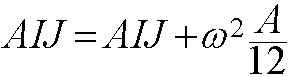 ;
;
end
BAND(iGlobal, Bcol)
= BAND(iGlobal, Bcol) + AIJ
End % (J loop)