ME 3901 Engineering Experimentation
Mechanical Engineering Department
Worcester Polytechnic Institute
Statistical Analysis of Experimental Data
· Uncertainty Formulation
· Averages and Least Square Deviations
· Uncertainty of a Mean
· Chi-Squared Test
· Gaussian Distribution
· Chauvenet’s Criterion
· Least Squares Linear Regression
Statistical Analysis of Experimental Data
Most “Results”
are obtained from multiple measurements of different parameters (length, width,
height, mass, etc.).
The
“Uncertainty” of this result is a function
of the uncertainties of each parameter used to obtain the result. Hence, one expresses the uncertainty of
the result wr, in
terms of the uncertainty of the independent measurements, wi
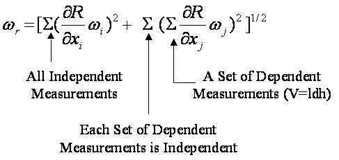
How does one determine the uncertainty
of each individual parameter?
Manufacturer
Accuracy/Precision Statements
The least
count (or half that) of the scale
The standard
deviation of a set of measurements used
to determine the parameter value.
Frequently, it
is desired to obtain the ‘average’ value of the parameter. What is
the average? There are 3 generally
accepted definitions of average: the mean, median, and mode.
Arithmetic Mean: 
Deviation: di = Xi - Xm
Standard (root-mean-square)
deviation
Population Biased 
Sample Unbiased 
![]()
Generally, if N > 20, then
the difference between population and sample standard-deviation values is small
and the population statistics can be used.
Example: What is the
uncertainty of the arithmetic mean?


The uncertainty of the mean
is: 
Median – the
‘Middle’ value of all ranked readings


Mode – the ‘most
frequent’ value of all readings.
Primary applications for
Median and Mode include:
Field
measurements,
Contaminant
measurements
Sometimes alternate
“means” are required.
Geometric Mean
Phenomena
which grow relative to itself, i.e. population statistics

The ‘arithmetic
mean’ is the most common statistic used when reporting a parameter
value. The standard deviation is a
quantifiable statement about the spread of parameter values taken to obtain the
mean. This variation in parameter
readings can be expressed in terms of probability.
Probability
If “Independent”
events occur the probability of all events is the product

Ex: What is the probability that 3
consecutive rolls of a die (pl. dice) will each land on 6?

It is advisable not to rely
on one measurement, but rather to carry out repeated measurements. If the die were
rolled repeatedly and measurements plotted a histogram can be created which
plots the frequency of occurrence relative to the bin.
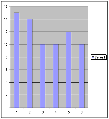
In this situation, one would
expect all 6 bins to be roughly equal.
Are they? This is a decision
frequently required in engineering experimentation. That is, one assumes the probability of
rolling a ‘1’ is the same as rolling a ‘3’, etc. But chance can effect this
‘perfect’ assumption and one must decide if the ‘dice’
are loaded.
A Chi-Squared
test is used to answer the question.

where M = number of groups (not trials). Frequency is used extensively.
Consider the previous
histogram situation: roll of die à 71 trials, expect about 12 occurrences

One uses Chi-Squared value
with a degree of freedom value, F, as in Table 3.6 of the Holman text.
F
= M – K
where K = constraints or restrictions, M = groups
In this case, F = 6-1 and P ~
0.83 which would indicate that the observed data was a reasonable outcome for
the expected value.
M = 6 for the possible die
outcomes and K=1 since our only constraint was that we had a fixed number of
samples.
Generally, expect: 0.1< P
< 0.9; otherwise, suspect foul data.

Frequently, one is measuring a parameter with an
expected single answer, such as the length of a table top. However, each time one measures it there
are slight differences in the length.
When plotted as a histogram the results might look like:
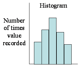
Gaussian Distribution:
If more and more measurements
were performed and the cells made smaller such that ![]() , then a distribution function would result.
, then a distribution function would result.
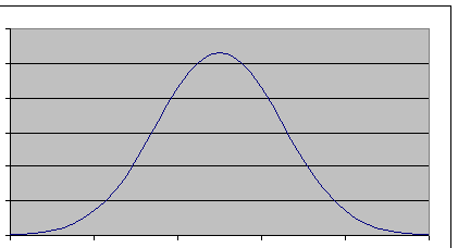
The shape of the distribution
function can be ‘normal’, i.e. bell-shaped. The function could be skewed or
multi-modal behaviors might exist. As with the roll of the die, is a
distribution function considered normal despite some shape
‘anomalies’?
A normal (or Gaussian)
distribution gives the probability of a measurement and is expressed as:

The coefficients are designed
such that when integrated over the entire possible range of data the
probability sums to unity:

Note: when x = xm the e() term drops
out and the maximum distribution function value is:

which occurs at the mean location.
Generally, one is interested
in knowing the probability that a value will exist within a banded window. Frequently, this window can be expressed
in terms of the mean and std. dev.

with 
and x1 is the deviation from the mean.
In this form, standard tables
exist such as Table 3.2 of Holman text:


Note that h1 is the
‘number of standard deviations’ about the mean. For h1 = 1, the table states that 68.3% of the data would
lie within one std. dev. of the mean.
Study this Table 3.2 (taken from
Holman class recommended text) and be sure you can use it. One should be able to determine the
percentage of expected values between 1 < h1 < 2, for example.
A set of data
contains some points that “just don’t look right”. However, one cannot eliminate data
without having some justifiable cause for the removal of data. Chauvenet’s criterion states that if the probability
of occurrence is less than 1/(2N) then the data
point(s) can be rejected. This
decision can be determined by calculating the h1 value knowing the std. dev. Then using Table 3.2 find the
probability, P, that an observation would range between – h1 and + h1. If (1-P) < 1/(2N)
then discard the point(s). Once
this procedure is performed and any questionable points eliminated, a new mean
and std. dev. are calculated. This
criterion is not iterative. That
is, one does not repeat the procedure based on the new mean and standard
deviation values.
The
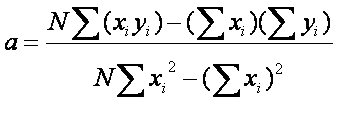
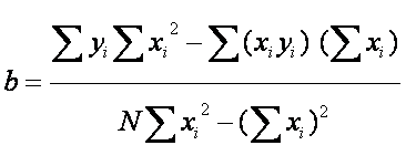
method of least squares is also used for curve fitting:

Want the line equation to
have a minimum least square error:

There are only 2 parameters (a and b) that can be adjusted to minimize the error. The minimum will occur when:


![]()


Two equations in 2 unknowns (a and
b). Solving for both:
How well does the regression
line fit? Similar to a standard
deviation of a mean, we have the standard error estimate of Y

The N-2 is due to two degrees
of freedom used in determining the regression line (the a
and b constants).
A correlation coefficient, r,
is used frequently to describe the goodness of the fit:
