There is still one more property of electric potential, namely potential difference, that you will work through because it is so directly relevant to lecture discussions about the electric potential. Due to the fact that the electrostatic field is a conservative field, the potential difference encountered in moving from one point to another depends only on the location of the end points and not on the path followed from start to finish. Add to that the fact that electric potential is a scalar quantity, potential difference promises to be easy to work with. There is one complication, and that is the fact that charge polarity must be taken into account because charges come in positive and negative varieties.
Another important property is capacitance, or the ability of an object to hold an electrical charge. A capacitor is an important electrical component that can hold separated amounts of positive and negative charges. Capacitors are as common in many electrical circuits as resistors. One important task to learn is the set of rules for determining the equivalent capacitance of a set of individual capacitors in parallel and/or series arrangements with one another.
Calculate the potential at a +1 point charge (1.00) and at a second point one grid length directly away with a +0.5 charge (0.50). Now, calculate the potential difference associated with moving from the first point to the second. Remember that a potential difference between two points is always defined to be Vfinal – Vinitial [Page 762, 13th edition of Young and Freedman].
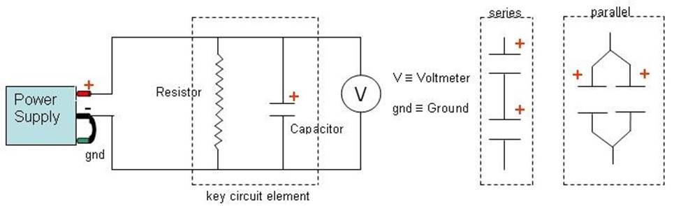
The resistance of carbon resistors is relatively easy to measure, as you learned in the previous experiment, the direct measurement of capacitance requires special equipment that we are not going to duplicate at some 30 separate PH 1120 lab stations. You are going to use a special approach especially suited to our Vernier equipment, with the emphasis on measuring the equivalent capacitance value of parallel and series combinations of capacitors as discussed in lecture. Note that the voltmeter is connect "across" the capacitor; it is in parallel with the capacitor.
As you will hear in lecture, a charged capacitor connected to a resistor discharges through the resistor in such a way that the voltage across the capacitor decreases with time according to the equation
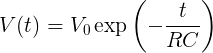
where V0 is the initial voltage across the capacitor at time t=0, R is the resistance value of the resistor, and C is the capacitance value of the capacitor. LoggerPro is able to plot both V(t) and ln(|V(t)|) = a – t/(RC) for some constant a.
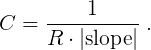
Whereas V(t) is an exponential, the natural log of the absolute value of V(t) is a straight line of slope magnitude

You will be using an R = 22,000 Ω ± 5% resistor in this experiment, and you will be measuring the slope of the natural log of the time-varying voltage across the capacitor, which means that you can solve for C as
Here is the procedure to follow: