 Introduction Introduction
|
Water loads are widely used in industrial systems of microwave heating. Conventional impossibility to convert all microwave energy into heat leads to the necessity to direct the energy not absorbed by the processed material to an efficient terminal load well matched to the system. The 915 MHz load designed and manufactured by The Ferrite Company, Inc. (FCI) consists of a short section (220 mm) of a WR975 waveguide connected to a circular metal tube (internal diameter 76 mm, length 435 mm) containing water (Fig. 1). It is used in the FCI 75 kW 915 MHz generators in one of the waveguide arms of the three-port circulator. This load is also available in the market as an independent unit for customized use. Originally, it was designed on the basis of extensive experimental development, which eventually led to a configuration providing excellent performance. However, this approach has not explicitly revealed major trends of the electromagnetic (EM) processes and has not suggested reasonable ways of possible modification and optimization of the load. The present study focused on computations was initiated as a response to the recently widened opportunities of comprehensive computer modeling of microwave heating [1]. The goal was to identify the circumstances of the stable and efficient operation of the load by systematically computing its major characteristics, particularly those which are either difficult to measure, or cannot be measured at all. To this end, the universal EM simulator QuickWave-3D implemented the conformal FDTD method [2-4] has been used. |
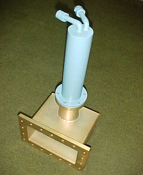 Fig. 1. 915 MHz high-power water load |
|---|
 Models
 Permittivity of Tap Water
Knowledge of the complex relative dielectric constant (DC) of tap water used in the load is critical for adequate characterization of the unit. The DC was calculated with the aid of the model based on the one described in [5] for saline water. The expressions for Re(DC) and Im(DC) derived from the Debye equation appear to be:
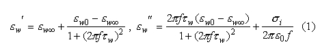
where eps0 = 8.854E-12 F/m is the absolute permittivity, f is frequency in Hz, epswoo is the high-frequency limit of epsw known to be independent on salinity [6] and equal to the one of pure (distilled) water, i.e., epswoo = 4.9. In (1), static dielectric constant of water eps0, relaxation time of water tau0, and the ionic conductivity sigmai can be expressed in terms of salinity of water Sw and temperature T as the following combinations [6, 7]:
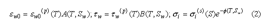
where epsw0(p) and tauw represent static dielectric constant and the relaxation time of pure water respectively, sigmai is the ionic conductivity of sea water at 25 C, and A, B, and phai are some empirical functions of Sw and T. By fitting to the experimental data obtained in [8-11], the parameters in (2) are represented as the following polynomials:
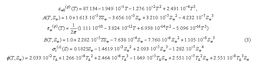
where Del = 25 - T. In (3), Sw and T are expressed in parts per thousand on a weight basis and degrees of C respectively. The data reported in [7-9] and implemented in the polynomials for and were measured for

respectively, so the model (1)-(3) is said to be valid under conditions stated in inequalities (4) [5]. Indeed, calculations of the DC for T > 40 C give non-physical results (Re(epsw) as increasing function of T). However, expansion of the range for Sw to cover smaller values of salinity (0.03-0.04) related to fresh water available from the tap appears to be possible.
Table 1 shows that in the range 0.3-3.0 GHz the agreement between the computed and measured DC is about 1% when salinity is known; the divergence may be larger when Sw is not specified. In addition to this, it is known that the polynomials for B, sigmai, and phai have been constructed in [6, 7] for 0 < Sw < 35. Thus, we conclude that the first inequality in (4) can be rewritten as 0 < Sw < 35. Consequently, this model can be applied for the computation of the complex DC of tap water at any frequencies and in the temperature range 0 < T < 40 C.
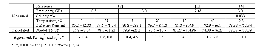
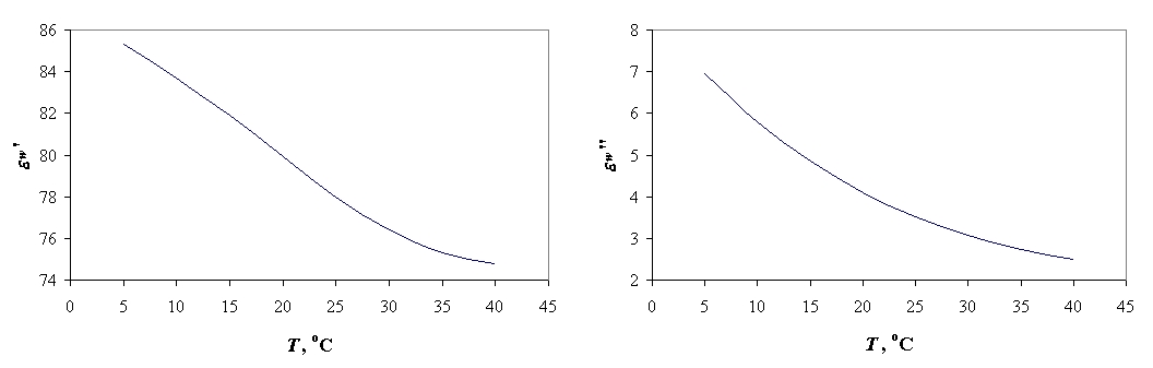
To determine Re(epsw) and Im(epsw) for the considered load, expressions (1)-(3) were used for f = 915 MHz and typical salinity of tap water Sw = 0.033. Fig. 2 shows that when T increases from 5 to 40 C, the real and imaginary parts decrease from 85.3 to 74.8 and from 7.0 to 2.5 respectively. Change in Im(epsw) appears to be very significant.
|
The Load Model in QuickWave-3D
The internal construction of the load has been described in the file of input data ("project file") for QuickWave-3D (Fig. 3). In the model, excitation of the circuit is assigned through the port simulating the presence of the dominant TE10 mode at the input waveguide cross-section of the load. About 4/5 of the length of cylinder (upper part in Fig. 3) is completely filled with water; water also occupies the thin-wall polystyrene cone located in the lower part of the cylinder and partially in waveguide section. Water is delivered to the load through one of the external water-pipes seen in Fig. 1 and further through the internal metal pipe inside the cylinder; it goes out through another external water-pipe. The model takes into account the parameters of the cone wall (relative DC 2.55, thickness 3 mm) and assumes the absorbing medium is uniform and unmoved (i.e., ignores water circulation within the load). To determine the magnitude of the signal within the cylinder, another port can be placed at some of its cross-sections; in Fig. 3, it is shown on the end. Since the upper part of the cylinder appears to be a coaxial line, microwave energy is primarily brought to the end of the load by the TEM mode, so this mode is assigned to the second port. The circuit was discretized into about 530,000 cells with typical cell dimensions from 6 mm (in the rectangular waveguide) to 2 mm (in the cylinder). A PC (Pentium III 450 MHz processor, 256 MB RAM, Windows NT 4.0) was used for simulations. |
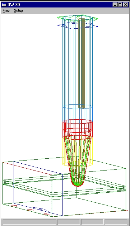 Fig. 3. 3D view of the load visualized in QuickWave-3D's Editor |
|---|
|
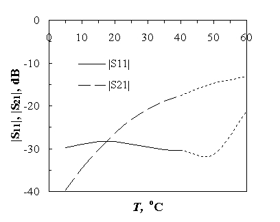 Fig. 4. Reflection
and transmission coefficients versus |
|---|
The graphs representing the transmission coefficient (|S21|) computed in the end of the cylinder (Fig. 4, 5b) show that the signal's magnitude varies with temperature: starting at about -40 dB for cold water, |S21| grows up to about -15 dB for hot water. Computation of the transmission coefficient at certain cross-sections of the cylinder allows us to determine where |S21| does not exceed the certain level. For instance, assuming |S21| = -20 dB is suitably small and non-affecting the circuit performance, the cylinder's length can be shortened by 25 mm.
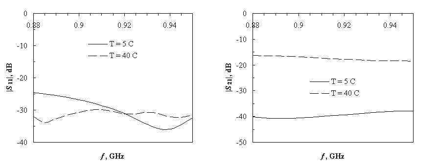 Fig. 5. Dispersion characteristics of reflection coefficient
(left) and transmission coefficient (right) |
|---|
|
Electric Field and Dissipated Power Typical patterns of the electric field (dominating component) and the dissipated power for a particular temperature of water are shown in Fig. 6. For other temperatures in the range 5 < T < 60 C, the field and power distributions are characterized by quite similar patterns. The absolute maximum of the field is located in the waveguide near the surface of the circular vertex of the plastic cone. Along the central axis of the cylinder, there emerge local field extrema with the magnitudes decreasing towards the end of the cylinder; the first maximum is characterized by the largest value. The pattern of the dissipated power has a sharp absolute maximum in the area of this extremum (close to the center of the polystyrene cone). For higher temperatures, the "hot spot" moves up a little bit. The suggested reduction of the cylinder's length is thus unlikely to affect the power pattern. |
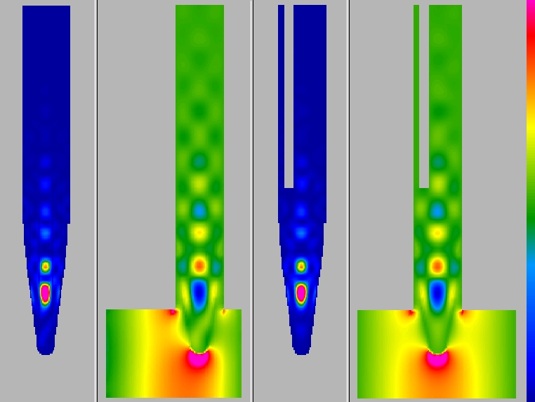 Fig. 6. Dissipated power (envelopes) and vertical
component of the electric field (instantaneous values) |
|---|
ConclusionThe conducted computer analysis has revealed the main reasons of the stable operation of the FCI 915 MHz water load: its level of matching and patterns of the dissipated power are not really sensitive to the temperature of water and possible deviation of the operating frequency. The length of the cylindrical part could be slightly reduced (by about 25 mm) without affecting the efficiency of the load performance as long as the water temperature is less than 50 C.
References The present web page is made on the
basis of the material presented at the 36th Microwave Power Symposium, San
Francisco, April 18-20, 2001