Finite Element Method

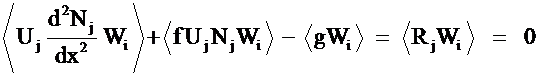
Consider an ODE of the form:

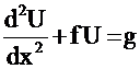
with the following Boundary Conditions:

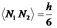
and

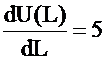
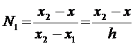
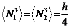
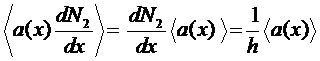
1.) Substitute for U an unspecified trial function into governing equation, i.e.

where

n = Number of nodes in system (or, locally, in element).

U_j = Unknown coefficients (to be determined), which are not a function of space, in general.

N_j = Known (user-specified) Basis function, which are a function of space, but not a function of time, in general.

2.) Force the Residual to zero in the global sense, i.e. satisfy the governing equation in the "weak form".

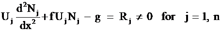
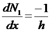
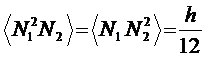
a.) Multiply by a Weighting function:

where W_i = Known (user-specified) Weight function.

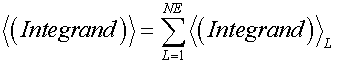
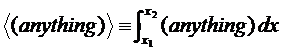
b.) Integrate (take inner product) over global domain and force to zero.

Definition of an Inner Product:

Implies that W is orthogonal to R

< ( ) > =

(dimensionally dependent)

If you can solve this equation then you have solved the governing equations, at least in the weak form.

3.) Discretize global domain into subdomains (Elements) such that S (Elements) = contiguous, non-overlapping representation of the global domain.

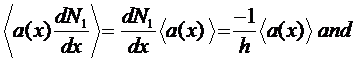
4.) Select a basis function for - a few helpful hints in this selection are

a.) select an orthogonal series basis function

b.) choose a computationally efficient series

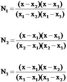
Ex. Lagrange Polynomials applied locally on each element

Assume Linear Element (N = 2)

Integration Formulae for 1-D Linear Elements

Assume Quadratic Element (N = 3)

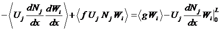
5.) Integration by parts:

Required for order PDEs using linear basis functions;
Provides a direct means to apply Boundary Conditions

more generally,

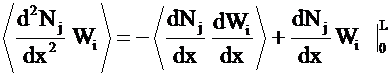
Adding in the other components of the ODE yields:

6.) Select Weighting functions

Ex: Choose "Galerkin"

(However, for clarity retain the W symbol. It will help when assembling matrices later.)

Note that for each weighting function, W_i, one must assemble all contributions from each basis function N_j.

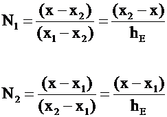
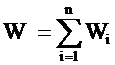
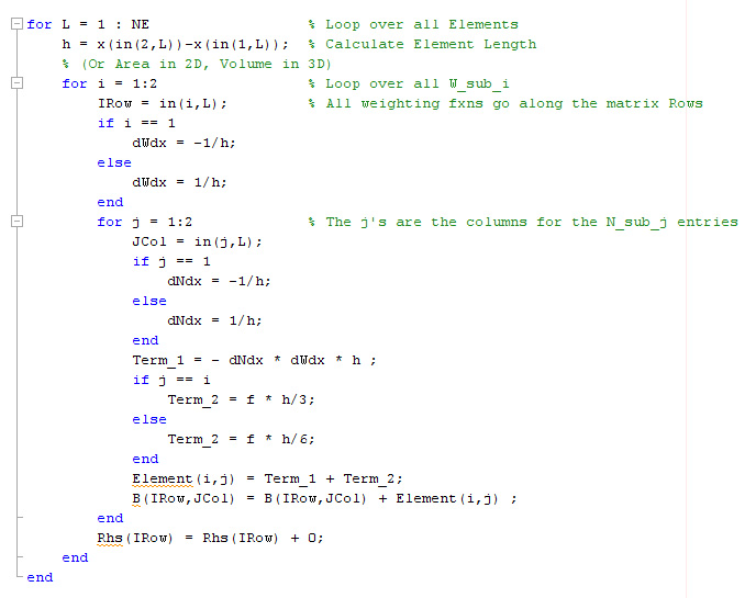
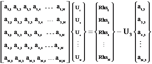
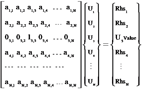
7.) Assemble Matrices – consider a single element, (Element L), and assemble all components associated with it. In general it will create a 2x2 matrix that will be inserted into the global n x n matrix:

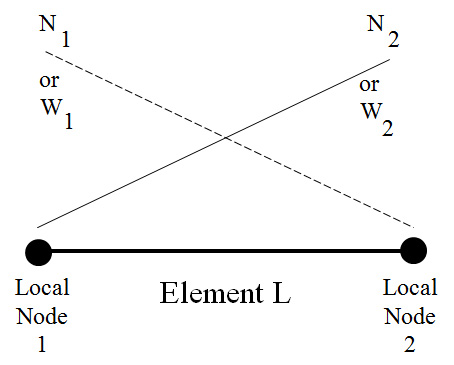
One row of equations for each W_i where i is locally 1 and 2.

One column of equations for each N_j where j is locally 1 and 2.

Note: the local definitions of Trial and Weighting functions specify that all N_j and W_i are zero
if they are not within the element. Consequently, we address the nodes OF THE ELEMENT as Local Node 1 and Local Node 2 for this two-node line element.

Refer to the Integration Table for all possible combinations of linear basis functions.

The 2x1 right hand side vector is:

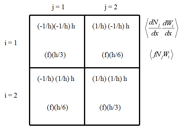
In general, we are forming an expression

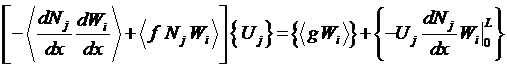
In a FE code: Loop over each element and assemble the local (elemental) contributions for the Lhs matrix [A] and the Rhs vector.

After this loop is completed, then (and only then) apply the boundary conditions to the set of equations.

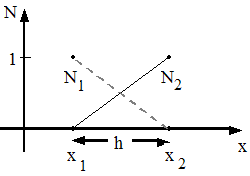
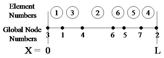
FE codes contain a lot of bookkeeping. One common mapping array is the element connectivity (or Incidence) list. It has the form:

IN(K,L) where

L = Element Number, L = 1, NE ( and NE = Number of Elements)

K = Local Node Number, K = 1, 2, … to the number of nodes in an element.

IN(K,L) = global node number ( maps global node number to the local node number within element L)

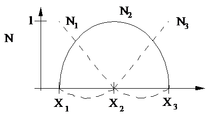
Consider the following 1-D example:

The Element number can have significance if using a frontal matrix solver.

The Node numbering can have significance if using a banded matrix solver.

Node and Element numberings have less significance if using a sparse, iterative matrix solver.

The mapping for this example is:

IN(1,1) = 3 IN(2,1) = 1

IN(1,2) = 4 IN(2,2) = 6

IN(1,3) = 1 IN(2,3) = 4

IN(1,4) = 7 IN(2,4) = 2

IN(1,5) = 5 IN(2,5) = 7

IN(1,6) = 6 IN(2,6) = 5

The FE approximation to the governing equation is accumulated (summed) in 3 nested loops (L, i, and j)

Everything done at the element level!

Easy to automate

a) One Element (problem-specific)

b) Assembly (problem-independent)

8) Add in the Boundary Conditions

a.) Type 1 BC : Satisfy Exactly U(0) = 1

(Note this is at global node number 3 for our example.)

One less unknown in algebraic system.

Remove row_3 and then move column_3 of matrix to Rhs since it is known (not usually done, but possible)

This process is somewhat cumbersome. It can change the bandwidth or structure of your system. It can cause other solution-solving anomalies if one is not careful.

Cleaner process:

Remove row 3 completely, i.e. place zeros in all entries.

Then place a 1 on diagonal of [A]

Put the solution (i.e. U(0)=1) into the Rhs

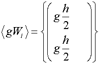
b.) Type II B.C. Satisfy approximately in {BCs} vector.

Recall: and for node 2 (in our example) the flux at the boundary is 5. Also note: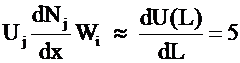

At the boundary node W_i = 1 for i = 2 (global) and W_i = 0 for all other nodes (including global node 7 which is part of element 4. The boundary condition is AT the boundary, not within the element.

Therefore to apply Type II Boundary Conditions in our example:

Rhs(2) = Rhs(2) – 5;

The entire formulation is complete. Call a matrix solver and obtain the solutions for U_j.