Finite Difference Methods

- Approximate the derivatives in the governing PDE using difference equations.

- They are useful in solving heat transfer and fluid mechanics problems.

- The methods work well for 2-D regions with boundaries parallel to the coordinate axes.

- However, they are cumbersome on curved and irregular shaped boundaries.

- It is difficult to write a general purpose computer program for the finite difference methods.

The Finite Element Method (FEM)

- Easily applied to irregular shaped objects

- Multiple materials (composites) are treated without difficulty.

- Mixed BCs can be applied

- General purpose codes for whole classes of problems can be written.

- The FEM combines several mathematical concepts to produce a system of linear or non-linear equations.  It has little value without a computer since equations range from 20 à 20K or more.

- The FEM is less stable (generally) than the FD method and it provides an integrated overall average of the solution set rather than explicit values at distinct locations.

There are 2 standard FEM treatment techniques:

a.) The Variational Method, and

b.) Weighted Residual Methods

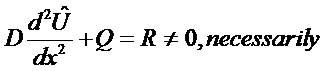
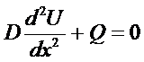
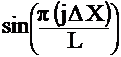
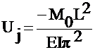
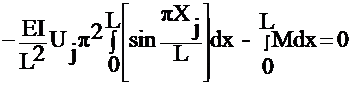
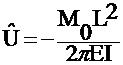
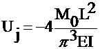
Using Calculus of Variation it can be shown that if:

1.) U = g(x) yields the lowest integration value of:

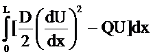
then

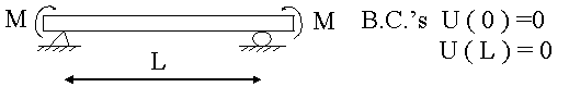
2.) U is the solution of the D.E.

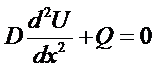
with BCs  U(0) = U₀ and U(L) = U_L

The term: 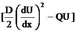   is the approximate functional.

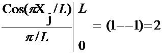
This solution strategy is NOT applicable for any D.E. containing first derivative terms.  The variational approach originated in stress analysis (during the 1950s) which involved even order derivatives only.  (Fluid mechanics traditionally use FDM for their solutions since the variational formulation was not valid for the Navier-Stokes set of equations.)

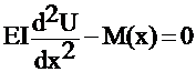
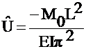
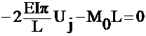
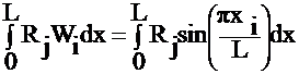
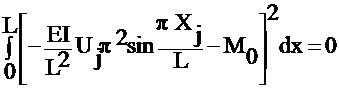
The Method of Weighted Residuals

Takes the governing equations

,   for example.

It approximates U with . Generally, this replacement of U with a guessed function is piecewise continuous, say

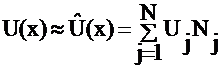
Where U_j are undetermined coefficients and N_j are the basis functions - which the user specifies or chooses.

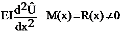
Since  does not satisfy the D.E. an error or residual results, i.e.,

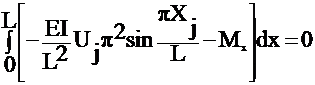
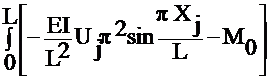
 The method of WR requires that this residual, when multiplied by a Weighting function, W, and summed over the region be zero.

òWR dx = 0

What we use for  and W distinguishes the various forms of  MWR

Recall: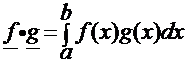               

is the definition of an inner product

Hence, if òWR dx = 0, it implies that R is orthogonal to W

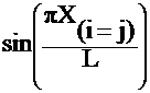
The 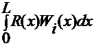 has i weight functions (1 for each node, in our case, or degree of freedom in system, formally)

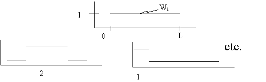
The common WR methods are:

i        Collocation

ii       Subdomain

iii      Least Squares

iv      Galerkin

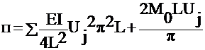
i.)  Collocation  =>     let W_i (x)  =  d( x- x_i)  

Then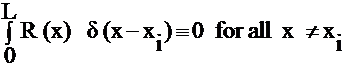      

                                       = R(x)  for  x = x_i

This requires that R(x) = 0 at specific points and if

The number of points = number of undetermined coefficients   \ a solution is available.

Ex:                 

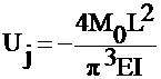
Let D =  EI ( resistance of the beam to deflection)

       Q = - M (the moment)

 

The solution of U = y displacement;

F.E.M.                    Replace U with a guessed function, say

Where U_j are undetermined coefficients and

Let N_j = basis function

=   or many other possible basis fxns

      Ex.  Lagrange Polynomials applied locally on each element

             

              

 

Exact Solution =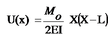 

Collocation:

Trial fxn: U  ~   Û = U_j N_j (implied summation)

=  U_j    where X_j = j*Dx

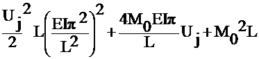
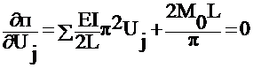
Plug into O.D.E.

 -  M_x     =    R(X_j)

Multiply by weighting fxn and integrate over Domain

Let X_i = L/2;  Then

  - M₀     =    0

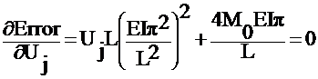
Solve for the unknown coefficient U_j

which multiplies the basis function for the final approximation of

 

ii) Subdomain

-       
Assume only 1 domain  i.e.

Same R(X_j) as with collocation

                                                       

iii) Galerkin:

Let  W_i=N_j

₌dx   =   0

Solving ,          same as Variational Method

iv)  Least Squares:

Error=

Minimize

 ;             

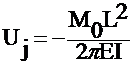
Variational Method:

P=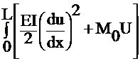 dx

approximate  

P=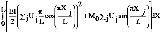

Minimize:

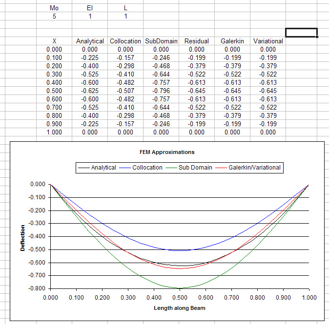
A small spreadsheet of the various methods:

FEM     SOLUTION      STRATEGY

   Variational Approach            Method of Weighted Residuals

Conservative Systems                   Use the PDE directly

Potential Energy of system                Guess a solution to U

    is Stationary                                  Apply a weighting fxn

                                  Integrate

    Functional                                  Require Residual to be

    Integrate                                              Zero Globally        

Algebraic Set of Equations

Apply Boundary Conditions

Matrix Solver

Solution