Last time:

a) Classify PDE in canonical form

b) Determine if given B.C.’s make the problem well posed

c) Examine analytical solutions ‘surrounding’ physical problem for comparison with numerical solutions throughout physical problem.

Today: Finite Difference Calculus

When a function U and its derivatives are single-valued, finite and continuous functions of x then by Taylor’s theorem:

Consider a 1-D situation with nodes uniformly spaced

Rearrange for

This is a first order approximation since the leading error term is of the ‘order’ h ~ O(h)

The finite difference literature defines to be the forward difference operator, i.e. so that:

A second order derivative can be found in similar fashion:

We want to solve for in terms of . Therefore, we must eliminate from the above equations. Multiply Eqn (6) by two and subtract from Eqn (7):

Rearrange for

or where

Generalizations:

and

That is:

n+1 points are required to represent with a leading error term of O(h)

Suppose one wishes more accuracy, i.e.

Write out the Taylor series:

We must eliminate to represent with O(h²) accuracy.

Multiply Eqn(11) by A and add to Eqn(10).

To remove the quantity (1+4A) = 0. That is, A = -1/4

Rearrange for

In general, n+m points are required to represent with a leading error term of O(h^m)

There is no restriction that one must use forward finite difference approximations. We can describe via

(16)

(17)

Multiply Eqn (16) by 2 and subtract from (17)

Rearrange for

Similarly, examine using a forward AND backward finite difference expressions

(18)

(19)

Subtract Eqn (19) from (18):

Rearrange

Note that for the same number of nodes, the central finite difference formulation is an order of magnitude more accurate.

Uniformly Spaced Finite Difference Coefficients (Taken from Hornbeck reference)

Consider what happens when the node spacing is not uniform

Examine the central difference formulation

In general: Loose an order of accuracy when mesh spacing is variable!

and the complexity of the formulation increases rapidly

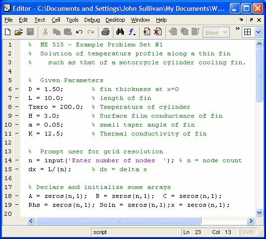
Example: Consider the heat transfer in a thin, slightly tapered fin attached to a chamber. The fin cools the chamber by radiation or forced convection, i.e. a motorcycle cylinder fin. Since the fin is thin, the temperature across its thickness is assumed constant. Determine the steady state temperature profile along the fin subject to the following boundary conditions.

T = T_s

at x = 0

where T_s = Tcylinder

dT/dx = 0

at x = L

The following 1-D O.D.E. can be used to describe this situation (Carslaw & Jaeger, pg 142)

Where

D is the thickness of the fin at x=0

a is the small angle of taper of the fin

K is the thermal conductivity of the fin

H is the surface conductivity of the fin

L is the length of the fin

The analytical solution for this problem is:

Where I₀, K₀, I₁, K₁ are modified Bessel functions.

The complexity is due to the coefficient (D-2ax)

However, a tapered fin is standard in Engineering Designs.

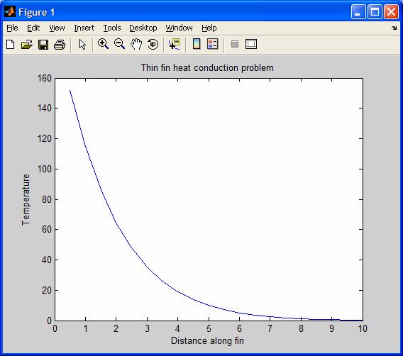
And we would expect the temperature profile to drop along the length of the fin.

How do we solve this system numerically?

Rewrite the O.D.E as:

Replace the continuous derivatives with the central finite difference approximations. Return to the Hornbeck tables and fill in the nodal subscripts.

Discretize the domain

Where Dx is constant.

Rearrange finite difference expression

For i = 1, 2, … n

This system of unknown equations requires a tri-diagonal matrix solver, i.e. the Thomas algorithm.

Where:

There are N equations and N unknowns, so it can be solved. Need to apply the boundary conditions.

At node 1 (Not the boundary):

But T(0) = T_s = known value, and

BdyCond(1)=0 since node 1 is not a boundary node

Therefore move the A₁T(0) to rhs which partially cleans up the lhs matrix:

Examine the equation at node N, which is a boundary node.

This formulation gives us an expression for the imaginary or shadow node (N+1). That is: T(N+1) = T(N-1) for the boundary condition to be true.

Now the lhs matrix has been corrected and the system of equations can be solved!

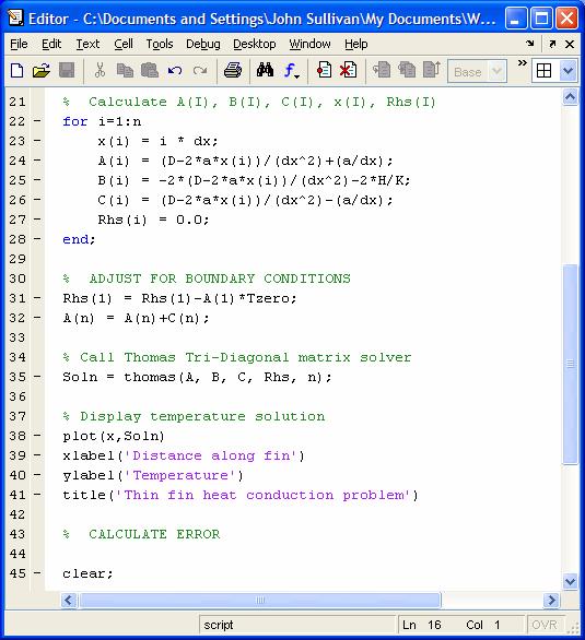
To solve, Calculate A(I), B(I), C(I), X(I), Rhs(I)

Adjust for the Boundary Conditions:

Rhs(1) = Rhs(1) – A(1)*T_S

A(N) = A(N)+C(N)

Rhs(N) = Rhs(N) + BC(N) = 0 in this case.

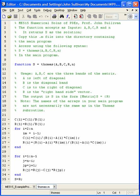
Call a tri-diagonal matrix solver, such as Thomas’ routine

Soln = Thomas(A, B, C, Rhs, N)

The temperature solution returns in the Soln(I=1 to N) array.

This tri-diagonal solver is incredibly efficient and short (only about 14 lines of code).

% ME515 Numerical Solns of PDEs, Prof. John Sullivan

% The function accepts as Inputs: A,B,C,R and n

% It returns S as the solution;

% Copy this .m file into the directory containing

% the main program

% Access using the following syntax:

% S = thomas(A,B,C,R,n)

% In the main program.

function S = thomas(A,B,C,R,n)

% Usage: A,B,C are the three bands of the matrix.

% A is left of diagonal

% B is the diagonal band

% C is to the right of diagonal

% R is the "right hand side" vector.

% The output is S in the form [Matrix]S = {R}

% Note: The names of the arrays in your main program

% are not necessarily the same as in the Thomas

% subroutine.

C(1)=C(1)/B(1);

R(1)=R(1)/B(1);

for i=2:n

im = i-1;

C(i)=C(i)/(B(i)-A(i)*C(im));

R(i)=(R(i)-A(i)*R(im))/(B(i)-A(i)*C(im));

end

for i=1:n-1

j=n-i;

jp=j+1;

R(j)=R(j)-C(j)*R(jp);

end

S=R;

How do we create a code to model this situation?

What are the basic, fundamental components of a code?

Go to the: [Next Lecture | Lecture Top | Previous Lecture ]