Leslie Population Models
Ma 2071
Problem: use
linear algebra to predict the growth and characteristics of a population which
is broken into age groups. This will
illustrate the numerical use of diagonalization. Conference yesterday
illustrated a geometric use of diagonalization.
Knowing the total population is good but knowing how it is distributed among different age groups
is better. Different groups have different social and economic needs which need
planning and resources for:
- young
children need daycare
- older
children need schools, playgrounds
- adults
provide taxes, have jobs, buy houses and consumer goods, and purchase
and drive cars
- older
adults require health care and different housing
- industries
need utilities, good roads and zoning
The general
study of these characteristics is called demographics. It is of concern to civil engineers who must
plan public utilities, computer scientists who provide information services,
mechanical engineers who design transportation media such as cars and trains,
electrical engineers who must provide adequate electricity, biotech people who
provide solutions to the unique health needs of each group, and mathematicians
(as actuaries) who work with various kinds of insurance needed by all groups
(auto, life, house, health). Electrical
and computer engineers also need markets for consumer goods they design such as
computer games, Internet access, high definition television and cell
phones.
In this course,
the Bio majors are looking at the spread of HIV and also what it might take to
effectively change that.
Quantitative
models are of considerable value.
Knowing in advance that the population of 20 to 30 year olds is going to
decline by 2% is of value to an auto manufacturer who has a line of sports
cars. In
______________________________________________
The mathematics: x is a
column vector with the size of the population for each group as its
components. In this hypothetical model,
the first component of x might be the number of 0 to 25 year olds, the second
component 26 to 50 year olds, the third 51 to 75 year olds and the last 76 year
old or more.
The future populations are generated according to the
matrix model
x(k+1) = A x(k)
A is called a Leslie Matrix. It has birthrates of each of the age groups along
the top row and has survival percentages along the subdiagonal.
It is 4x4 in this instance. I will use Maple to study
this below…
> with(linalg):
Warning, the
protected names norm and trace have been redefined and unprotected
> with(plots):
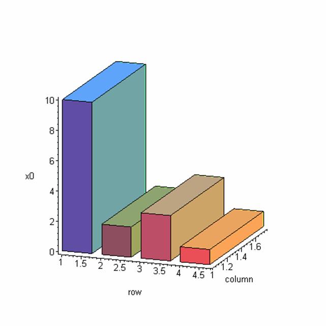
Intitial Population - divided into
4 age groups
(lots of young
people)
Warning, the name
changecoords has been redefined
> x0:=matrix(4,1,[10,2,3,1]);

This can be displayed in histogram form:
> matrixplot(x0,heights=histogram,axes=frame,gap=0.25,style=patch);
The following matrix is used to compute the population one
generation into the future.
> A:=matrix(4,4,[.2,1.5,.7,.2,.9,0,0,0,0,.88,0,0,0,0,.84,0]);
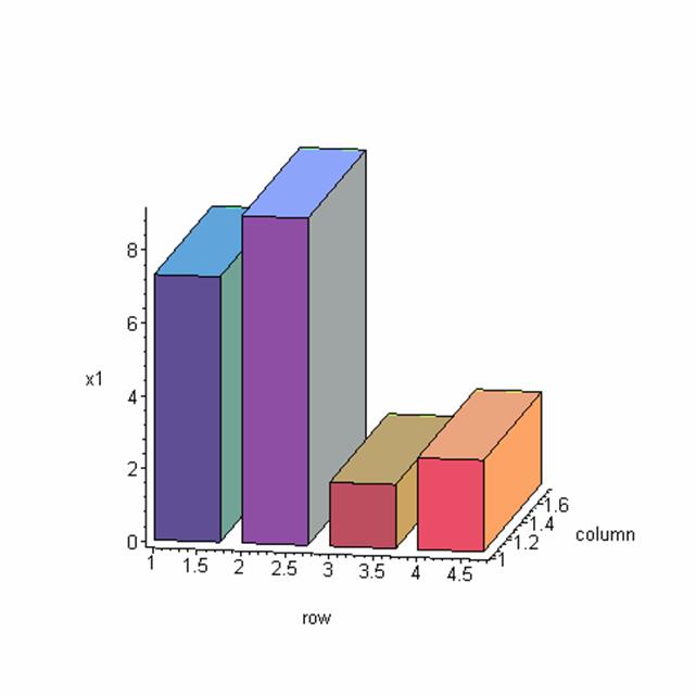
Transient Behavior - what happens in the immediate future:
![]()
> x1:=multiply(A,x0);

> matrixplot(x1,heights=histogram,axes=frame,gap=0.25,style=patch);
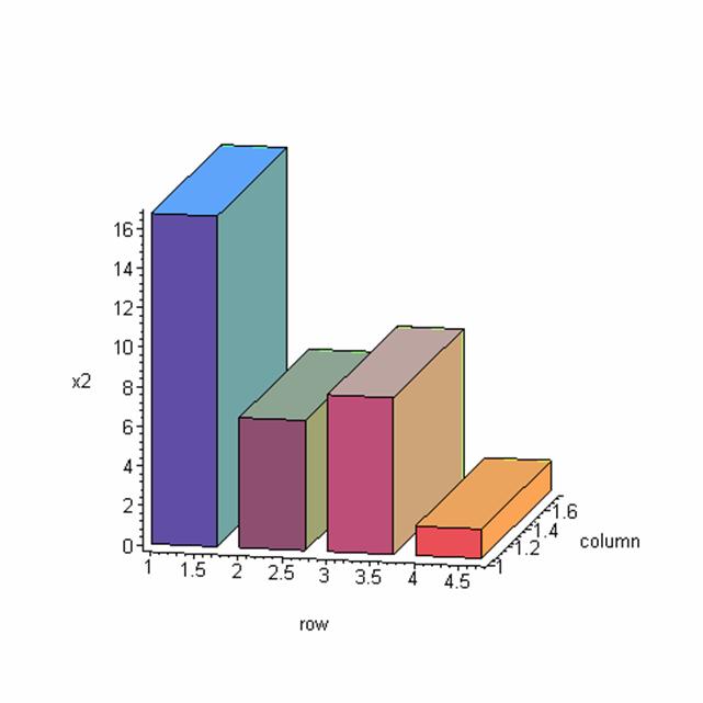
> x2:=multiply(A,x1); 2 units of time into the future
>
> matrixplot(x2,heights=histogram,axes=frame,gap=0.25,style=patch);
Now let's look further into the future; 10
units of time.
> x10:=multiply(A^9,x0);
> x11:=multiply(A^10,x0);
Let's compare how each component of the population has
changed:
> ratio1:=x11[1,1]/x10[1,1];
![]()
> ratio2:=x11[2,1]/x10[2,1];
![]()
> ratio3:=x11[3,1]/x10[3,1];
![]()
> ratio4:=x11[4,1]/x10[4,1];
![]()
Next, we plot both populations on the same histogram:
> P:=augment(x10,x11):
> matrixplot(P,heights=histogram,axes=frame,gap=0.25,style=patch);
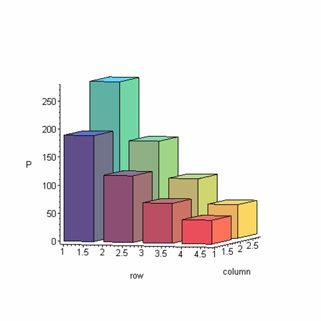
What does this last histogram show? It shows that the shape remains the same, from one period of time to the next. All groups increase in size but they increase
in size by the same factor (1.44)
What does this have to do with diagonalization? The vector made up of the sizes of the age
groups is an eigenvector of A. The
factor that they increase by is an eigenvalue of A, 1.45. More specifically, it is the
largest of the four eigenvalues of A, the dominant
eigenvalue.
What the above histogram shows is algebraically shown as
x(11) = 1.45 x(10)
and since
x(11) = A x(10)
this means 1.45 is an
eigenvalue of A and x(10) is its eigenvector.
Furthermore, this behavior continues indefinitely. This means x(21) = 1.45 x(20) or
x(25) = 1.45 x(24). In other
words, the shape of the histogram remains the same and the population increases
by a factor of 1.45 each time (i.e. goes up by 45%)
The moral? If we know the
largest eigenvalue and its eigenvector for a dynamical system, then we know
what the long term behavior of the system will be.
The profile of the solution will be determined by the eigenvector
The rate of growth will be determined by the eigenvalue.
These remarks apply to any dynamical system of the
form x(k+1) = A x(k).
All of this can
be quickly predicted by computing the eigenvalues and
eigenvectors of A:
> eigenvectors(A);
Amidst
this barrage of data is a largest eigenvalue, 1.444463... and its
eigenvector, [.79, .49, .3 , .175] Its components have the same relative size
as x(11) and x(10) above (you might check this with a calculator!)
To see why it
works out this way, we need to look at the basic equation A
= P D P-1 We will do that
Friday…