Fourier Transform of force.wav

Fourier Transform of Wave File

To begin the FFT operation we define n as the length of the wave minus 1 so that the equations that follow are easier to follow. We are subtracting 1 to eliminate the extra point that the length command creates when finding the length of the wave. To plot two arrays they must have the same amount of data points. Enter each of these commands into your own M-File or into the command window.

n=length(wave)-1;

Define f as the frequency domain array from 0 to fs by increments of fs/n. The increment is the sampling frequency divided by the number of points to be accounted for over the frequency range. This time around you notice that the values are in frequency (Hertz). The upper bound is the sampling frequency and the increment is simply the sampling frequency divided by a scalar amount resulting in Hz.

f=0:fs/n:fs;

Take the FFT (Fast Fourier Transform Algorithm) of the wave and set it as the variable forcefft for example. We take the absolute value of the FFT to remove the complex part of the transform so we are able to plot the function. We cannot plot complex values in the real number plane.

forcefft=abs(fft(force));

All that is left to do is to create another figure (so we do not plot over our previous plots) and plot the FFT of the wave by the frequency domain array f that we created above.

figure(2);

plot(f,forcefft);

xlabel('Frequency in Hz');

ylabel('Magnitude');

title('The Force FFT');

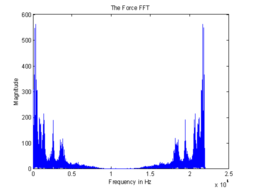
As you can see the FFT creates reflection in the plot. The higher frequencies are identical to the lower half. Disregard the reflection or click the +magnifying glass and drag over the part of the plot that is important.

Most of the frequencies are low, representing human speech. This plot could act as a footprint for speech identification.

Return to Wave File Analysis.