Regression Analysis

Definition: A statistical technique used to find relationships between variables for the purpose of predicting future values.

Goal: The goal of regression analysis is to determine the values of parameters for a function that cause the function to best fit a set of data.

In linear regression, the function is a linear (straight-line) equation.

In quadratic regression the function is a parabola.

In exponential regression, the function is an exponential curve.

Extrapolation: To estimate (a value of a variable outside a known range) from values within a known range by assuming that the estimated value follows logically from the known values.

Interpolation: To estimate a value of (a function or series) between two known values.

Least Squares: A method of determining the curve that best describes the relationship between expected and observed sets of data by minimizing the sums of the squares of deviation between observed and expected values.

Technology Pros and Cons:

There are pros and cons of using technology for computing regression. Some pros are that the user can be relieved from tedious computations, and can spend more time doing data analysis. A big con is that the user does not have to understand how the regression is computed.

Regression in the Secondary Curriculum:

Technology which can calculate regression can be very useful in the secondary curriculum. Some classes that it can be used in are Algebra and Statistics.

In Algebra, students could predict what they think is a best-fit line for a given set of data points, and use a calculator to verify their results.

Mathematical Foundation for Regression Analysis:

Given a set of data points, there may be a best-fit function which can be used to predict results. Some possible best-fit functions include linear functions (straight-line), quadratic functions (parabolic) or exponential functions (exponential curve).

Once the given data is plotted, visual inspection is useful to determine the type of regression analysis to use. Another method of finding a best-fit function is to use the various regression analysis programs and plot the outcomes to determine the best-fit.

Simple linear regression refers to fitting a straight-model by the method of least squares and then assessing the model. The method of least squares requires no assumptions. If we let the best—fit line be Y = aX + b, then the method of least squares finds solutions to the coefficients a and b by minimizing the sum of the squares of the vertical distances from the data points to the best-fit line. Let E be the sum of the squared vertical distances of the ’s from the best-fit line.

To minimize E, we must take the partial derivatives of E with respect to a and b.

By setting each equation equal to zero, we get the following system of equations.

By solving this system for a and b, we can find the equation of the best-fit line for the data in the form y = ax + b.

Similarly, the quadratic best-fit curve in the form y = ax² + bx + c can derived using the least square method. Again, let E be the sum of the squared vertical distances of the ’s from the best-fit quadratic.

To minimize E, we must take the partial derivatives of E with respect to a, b and c.

By setting each equation equal to zero, we get the following system of equations.

By solving this system for a, b and c, we can find the equation of the best-fit quadratic for the data in the form y = ax² + bx + c.

Similarly, the exponential best-fit curve in the form y = ae^bx can derived using the least square method. Again, let E be the sum of the squared vertical distances of the ’s from the best-fit exponential curve.

By taking the natural log of both sides we get . If we let , then is linear. Therefore, we can do the same as above for the linear best-fit line to find a and b.

How Good is the Fit?

Correlation coefficient

R is the sample correlation coefficient. It measures the extent of the plotted points clustered about a best-fit model equation. The correlation coefficient can be from -1 to 1 inclusive. If the value of R is close to 1, then the data would suggest a positive relationship. If the value of R is close to -1, then the data would suggest a negative relationship. If the value of R is close to zero, then the data would suggest no relationship. However, the correlation coefficient can be misleading. A visual inspection of the plotted data should accompany the correlation data analysis. It is important not to confuse the correlation coefficient with the slope of the best fit line, they are not the same.

R is the sample correlation coefficient. For linear correlation coefficient, R is the sum of the products of the two standardized variables divided by one less than the number of data points.

Another version of R is

In simple linear regression, the square of the linear correlation coefficient, R², is the proportion of the variation of the response variable, y, explained by the straight-line model. Example, if R²= .84, then we can say 84% of the data is explained by the linear model.

Example of simple linear regression

The following is housing data for Sturbridge new construction on 1 acre lots, the axis are square footage vs. cost in thousands.

Square Footage	Cost in Thousands of Dollars
1750	239
1872	289.9
2100	299.5
2024	324.9
2600	432.9
2688	339
2740	404.9
2780	410
2900	459.9
3400	589.9

The following is a scatter plot of the data.

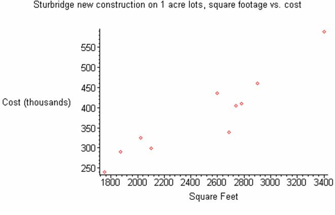
From a visual inspection, the data appears to be linear. Using the simple linear regression techniques described above, we get the following linear model.

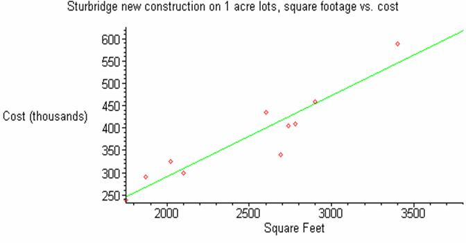The following is a graph of the data and the linear model of the data.

The best-fit linear model appears to be a very good representation of the data. Next, we will calculate the linear correlation coefficient using the equation above.

Since R is very close to one, it suggests that the data has a strong positive linear relationship. In other words, the linear model is the appropriate model for this data. Next, we will calculate R².

This value suggests that about 87.6% of the data can be explained by the linear model.