Regression Analysis is a method of taking some measured data and describing an equation and graph that seems to best fit the measured data. By fit we mean the graph appears to go through the cloud of data points in such a way that it balances the data points above and below the fitted line. All measurements involve some error and deviation due to issues such as:
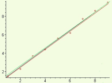
These three lines are not that different, but which is more accurate than the others at going through the data and enabling us to predict values for of whatever is being measured for domain values of 4.5 and 7.5, where there are no measurements? Is there another line that is more accurate? This is the domain of regression analysis: a systematic approach with a rational basis for estimating a best graph for some data.
We now examing the reasoning and mechanics
behind finding the line of best fit that produces a set of ordered pairs
corresponding to each domain value existing in the measured data set so
that the overall difference between the predicted and actual range values
is minimized.
Mathematical Foundations of Regression Analysis
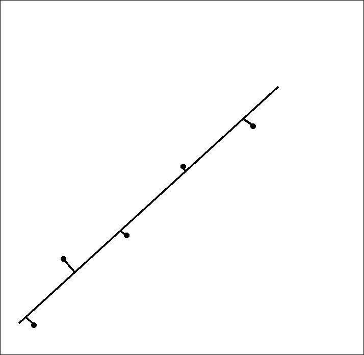
The degree to which the predicted values of a line that tries to express the trend of the some data varies from the actual measured data values is the key concern of regression analysis. Given such a line, how close it fits to measured data points can be measured by the distance between successive data and said line.
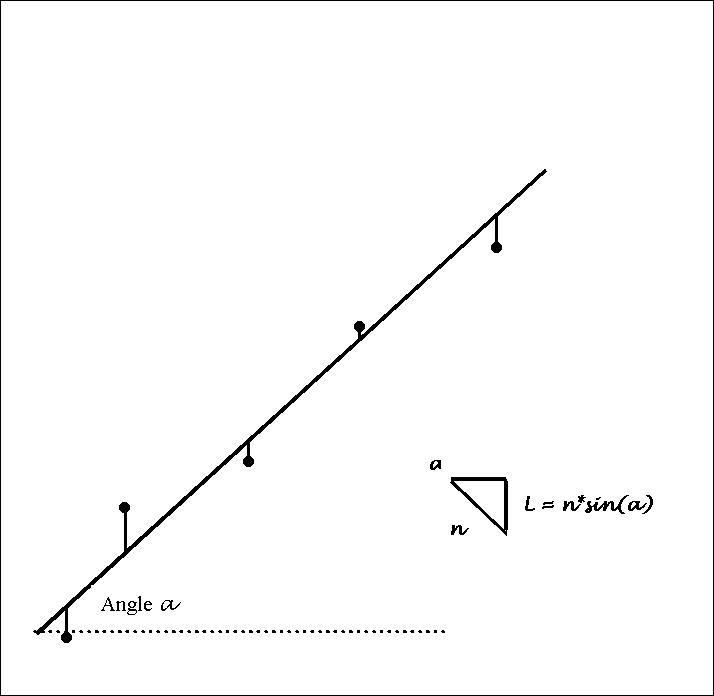
If the length of each normal line
from proposed fit lines to each data point is somehow collectively minimized,
that which has the least variance would be the best fit. Rather than the
normals, the lines that are collectively minimized are vertical lines from
each data point to the line. This is convenient because the domain values
are then identical, and mathematically equivalent, as these distances lare
each are each equal to to the length of the normal, n
divided by the sine of the angle between the line of fit and the horizontal:
l
=n/sin(a)
Summing up each of these vertical variances would yield a value a Total Deviation = S(yl -yi.) [where for each x-value in the measured data set, ylis the y-value on the fit line and yi. the measured value. However, since the cancellation of some upwards variences by douwnward signed ones might be arbitrary with respect to minimizing overall variance, using the absolute value might be a better value to minimize for various candidate fit lines: Absolute Deviation = S|yl -yi.|. Still another approach to eliminating the sign for a summed variance is to square each difference, yielding the most common such measure: Squared Deviation = S(yl -yi.)2.Averaging this measure over the number of measured data points yields Variance =S(yl -yi.)2/n, and taking the square root of this defines the Standard Deviation of the data fit between the measurd data and fit line: Sy=
In order to analytically derive the line which minimizes Sy, we note that that line can be described by yl =mxl +b, where m and b are respectively the slope and y-intercept of the line of best fit. Thus the variance S(yl -yi.)2/n = S(mxl +b-yi.)2/n. Minimizing the summation may be approached by using the calculus. We take the derivative of S(mxl +b-yi.)2 with respect to m & b, and by setting the equations equal to 0, define critical points of S(mxl +b-yi.)2:
Since each xl is a domain value on the best fit line identical to that in each ordered pair of measured data (xi. , yi.) , we merge the indexes, and by setting each partial derivative equal to 0 and rearranging, we describe the sought for minima by:d/dmS(mxl +b-yi.)2 = 2S(mxl +b-yi.)xl and d/dbS(mxl +b-yi.)2 = 2S(mxl +b-yi.)
We then solve these two equations simultaneously to find best fit line y = mx + b which minimizes Sy=mSxi.2 +bSxi.=Sxi.yi.
mSxi + bS1 = Syi.
What About Exponential & Quadratic Models vs Linear?
Now that we've explored how to best fit an equation to some linear data, we shall explore how to do the same for data sets exhibiting exponential or quadratic growth patterns.
For data appearing exponential, we need find a and b such that y = aebxis optimized to the data in a manner analogous to that just explored for linear data. Taking the natural logrithm of each side yield lny = lna + bxlne or:
We then solve for b and lna after the manner of m & b in the linear model:lny =bx +lna
and, after solving simultaneously for lna and b, use these to describe the best fitting model describing the exponential data:bSxi.2 +lnaSxi.=Sxi.yi.
bSxi + lnaS1 = Syi.
For data requiring a quadratic fit, y = ax2 ...y = elna+bx
How Good a Fit? The use of r/r2
Once we have found a linear equation that best fits some data that appears to be generally linear, how do we describe just how linear the data is in the first place?
For a given set of measurements (xi. , yi), the averaged sums of the deviation of each data point's coordinate values xi. and yi from their respective mean values x and y , (xi -x) and (yi-y) will yield the the standard deviations of the data sets:
If we normalize the actual raw xi. and yi data to its respective mean values x and y, so as to shift the origin by <-x,-y>, we have modified the measured data to (xi -x ,yi-y) so that its mean is (0,0). If we then further normalize the thus modified data to the respective x- and y-standard deviations, Sx and Sy , the two scales are more in proportional to each other, we can measure how well correlated the data is by:Sx=S(xi -x)2/n and Sy=
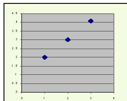
If we had a set of data {(1,2),(2,3),(3,4.1)}, which is almost a straight line with a slope of close to 1,S[(xi -x)/Sx][(yi-y)/Sy]
this calculation would yield a correlation of approximately 0.9996:
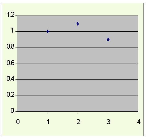
While the data set {(1,1),(2,1.1),(3,0.9)} would yield Sx= 0.8165 , Sy = 0.0816 , and Correlation = 0.5Sx =
Sy =Correlation = (1/3)[(1-2)(2-3.033)+(2-2)(3-3.033)+(3-2)(4.1-3.033)]/[(0.8165)(0.8576)] = 0.9996
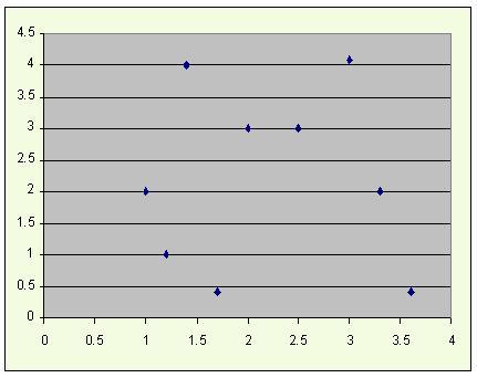
and a very loosely bound set of data with little or no apparent linear pattern, such as
{(1,2),(1.2,1),(1.4,4),(1.7,0.4),(2,3),(2.5,3),(3,4.1),(3.3,2),(3.6,0.4)} yields a correlation of only -0.0221
In sum, this measure seems to be nearer to 1 for a perfect positive correlation to linearity, and close to 0 for little or no linear correlation. This measure, the linear correlation coefficient, is usually designated with a small r.
x
x
An Application of your choice
Technology: pros and cons of various pieces of technology
The Secondary Curriculum: where might this fit in; suggestions
Appendix: Terminology for the Novice
regression
least squares
interpolation
extrapolation