Wave File Analysis: Specific Tone

Using the same steps that were used to plot the force.wav file in the time and frequency domain, we can analyze a tuning fork recording. Given tune.wav lets import it into the Matlab workspace, plot it in the time domain, take the Fourier Transform of it and look at that plot in the frequency domain to find out what frequency our tuning fork recording really is. Right click on tune.wav and save the file to your desktop so that the wavread command below is valid.

Step One – Opening the Wave File

Just getting the WAV file located and open in Matlab is not an easy task! You have to know where the file is located. Obviously if you can’t get it open, you can’t do any Fourier analysis of it! Furthermore, things change depending on what operating system you are using. What follows are step by step instructions, depending on the OS.

We will once again use the wavread function to import the wave file. Enter all of these blue italicized commands into your own M-File, located under file, new, m-file. Opening the wave files is tricky for the different windows operating systems.

Under Windows 95/98:

[wave,fs]=wavread('c:\windows\desktop\tune.wav');

Under Windows NT/2000/XP:

[wave,fs]=wavread('c:\Documents and Settings\USER\Desktop\tune.wav');

note: Your personal login id must replace USER.

How will you know if you did not open the file correctly? You will get a message comparable to:

??? Error using ==> wavread

Cannot open file.

At that point, recheck the path of the wave file in the wavread command and correct it!

Step Two – Using the Wave File

OK – now you have the file within your sights, you can actually go about analyzing it with the Matlab tools. What follows illustrates that.

To play the wave file we will use the sound function.

sound(wave,fs); (try this!!)

Now we want to look at the wave file in the time domain. That means we want to see the sound data plotted over time in seconds. To do this we will need an array t (for time, makes sense!) that contains the correct number of points to represent the wave file.

Here is the setup for the time domain array from 1 to (length(wave)-1)/fs, by increments of 1/fs. The variable fs is the sampling frequency or the number of samples per second. The 1/fs is expressing the increment, note that one divided by the sampling frequency leaves us with a number in seconds. The upper bound is the number of data points divided by the sampling frequency. The result is the total amount of seconds contained in the wave file.

t=0:1/fs:(length(wave)-1)/fs;

We have done most of the work now, just need to setup the plotting commands. Create a new figure window with the figure command. This will isolate this plot to its own window. Next plot the wave by the time domain array t that we created above. The title, ylabel, and xlabel commands create the title, and axes labels on the plot after it has been plotted.

figure(1);

plot(t,wave);

title('Wave File');

ylabel('Amplitude');

xlabel('Length (in seconds)');

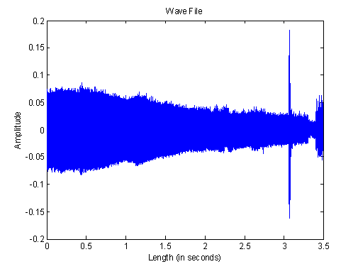
This yields the continuous time plot of the tuning fork recording:

Now we want to carry out the Fourier Transform of the wave file, plot the transform in the frequency domain and then rescale the axes so we can see exactly what frequency our tuning fork recording was.

We define n as the length of the wave minus 1 so that the equations that follow are easier to follow. We are subtracting 1 to eliminate the extra point that the length command creates when finding the length of the wave. To plot two arrays they must have the same amount of data points.

n=length(wave)-1;

Define f as the frequency domain array from 0 to fs by increments of fs/n. The increment is the sampling frequency divided by the number of points to be accounted for over the frequency range. This time around you notice that the values are in frequency (Hertz). The upper bound is the sampling frequency and the increment is simply the sampling frequency divided by a scalar amount resulting in Hz.

f=0:fs/n:fs;

Take the FFT (Fast Fourier Transform Algorithm) of the wave and set it as the variable wavefft for example. We take the absolute value of the FFT to remove the complex part of the transform so we are able to plot the function. We cannot plot complex values in the real number plane.

wavefft=abs(fft(wave));

All that is left to do is to create another figure (so we do not plot over our previous plots) and plot the FFT of the wave by the frequency domain array f that we created above.

figure(2);

plot(f,wavefft);

xlabel('Frequency in Hz');

ylabel('Magnitude');

title('The Wave FFT');

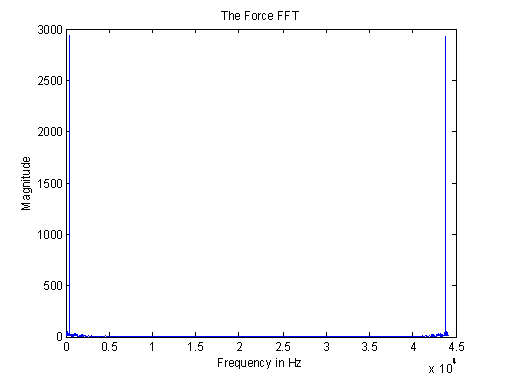
This yields a plot showing us the exact frequency of our tuning fork.

It appears that the FFT creates a reflection. The same data has been repeated in the higher frequencies. This is repetitive information that we should disregard. We can simply zoom in by clicking the +magnifying glass and dragging the mouse over the plot of the area that we want to see or change the axes properties shown below.

Step Three – The Final Result

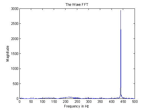
As you can see there is one distinct frequency of our tuning fork. All we need to do now is change the x axes range to accurately view that frequency. In Matlab go to edit then axes properties and uncheck the auto for the x axes and change the upper bound of 45000 Hz to 500 Hz for example. Now click ok and your plot has changed to something like this:

In this plot we can clearly see that the tuning fork frequency is around 440Hz. We have completed what we set out to do. Congratulations!!!

NOTE TO NEW USERS OF MATLAB:

If you are trying to get started with all of this and want the bare minimum of code it takes

to analyze a wave file, the discussion above can be compacted into the following code (with

comments colored ) which is highlighted in yellow:

Note: This assumes you have used the "cd" command (change directory) to

move to the directory (folder) where your file is.

(You can save time by cutting and pasting from here to Matlab as opposed to re-typing. You have to do it one line at a time – Matlab is an interpreted language)

>>[wave,fs]=wavread('your_file_name.wav'); /* read file into memory */

>>sound(wave,fs); /* see what it sounds like */

>>t=0:1/fs:(length(wave)-1)/fs; /* and get sampling frequency */

>>plot(t,wave); /* graph it – try zooming while its up…not much visible until you do*/

>>n=length(wave)-1;

>>f=0:fs/n:fs;

>>wavefft=abs(fft(wave)); /* perform Fourier Transform */

>>plot(f,wavefft); /* plot Fourier Transform */

now go into the plot you have generated and use the "zoom" feature to see what the frequency is that you are looking for. Simply looking at the graph will get you little information.

Comments on moving around among folders in Matlab:

Matlab is a Dos oriented language and predates Windows. Dos used “directories” instead of “folders”. The "cd" command is for "change directory". Essentially the same as in Unix. You either >cd folder_name

to go down into a folder or > cd .. to go up one level. Also " \" stands for the root directory so doing >>cd \ puts you there.

If you try to use a folder name which has blanks in it, put the whole folder name in single quotes:

>>cd 'My Matlab Files' (or it will not parse and you get an error)

The command "dir" will list files like "ls" does in Unix

It accepts qualifiers such as: >>dir *.wav which will only display files ending in .wav

____________________________________

Return to the Matlab Tutorial.